Analyze Performance Report
Once the profiling report is submitted, the system will automatically run the performance estimation against all the currently supported architectures and generates a performance report.
The performance report shows a roofline chart for each analyzed architecture (shown in different colors). The user can hide/show each roofline chart by clicking on the corresponding label inside the legend above the charts area.
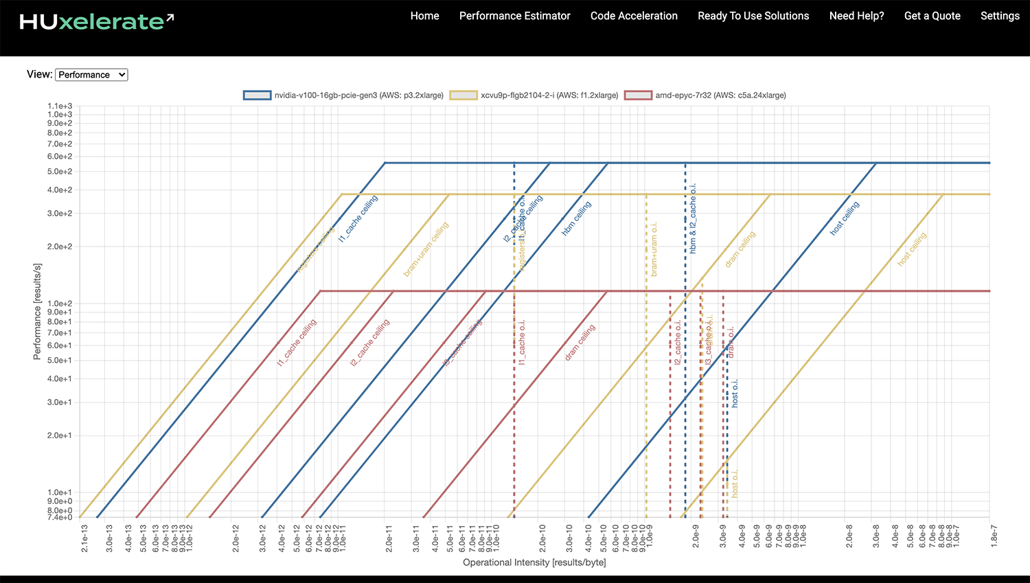
Roofline chart
The Y axis reports performance measured as results/s (i.e. the number of results generated per second), while the X axis reports the operational intensity expressed as results/byte (i.e. the number of results for each byte moved to/from a given memory). By default a result corresponds to a complete execution of the profiled function. Hence, a performance value of 100 results/s means that the profiled function can be executed 100 times per second.
The Performance Estimator also support user-defined result metrics. If you need to define a custom result refer to this section.
For each architecture an horizontal line (parallel to the X axis) is shown. This horizontal line represents the peak performance value that the profiled function could achieve on the given architecture. The peak performance is computed considering the type of operations performed by your function and the compute capability of your hardware but, does not consider possible bottleneck due to data transfer.
An architecture usually consists of several memories, each with its own peak bandwidth and size. When dealing with accelerator cards such as GPU and FPGA connected via PCIe to a host system, the host memory and the data transfer to/from the host memory must be considered. The Performance Estimator assumes that all the input/output data of the profiled function resides in the main memory of the host system.
To understand whether performance might be limited due to data transfers, the roofline chart provides memory ceilings and operational intensity values. Memory ceilings are slanted lines that represents the peak bandwidth of a given memory (memory names are shown close to each line in the roofline chart). Memory with higher bandwidth will have memory ceiling close to the left side of the roofline chart, whereas, memories with lower bandwidth will have their memory ceiling closer to the right side of the roofline chart.
The tool estimates a lower bound of the average data transfer to/from each memory of the architecture to compute a single result. The inverse of this value, that is, the number of results per byte transferred to/from a given memory (results/byte), is the operational intensity with respect to that memory, which is shown as a vertical line labelled with the corresponding memory.
A high operational intensity value means that the profiled function spends relatively more time computing data than moving data to/from that memory. A low operational intensity value means that the profiled function spends relatively more time moving data to/from the memory than doing actual computation.
In order to understand if a data transfer to/from a memory can be a bottleneck, you need to look at the memory ceiling and the operational intensity for that memory.
If the operational intensity is completely to the right of the memory ceiling, i.e. there is no intersection between the memory ceiling line and the operational intensity line, the function is compute bound with respect to that memory and there are no performance penalties.
If the operational intensity line and the memory ceiling line of a memory intersect, it means that the profiled function is memory bound with respect to that memory. In this situation, the maximum performance cannot exceed the performance value at the intersection of the two lines. In other words, it means that the time spent transferring data to/from that memory exceeds the time spent in doing useful computation.
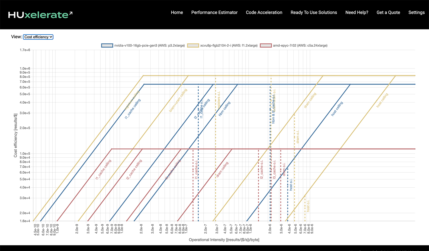
Cost efficiency view
In the top right corner of the roofline chart, it is possible to switch from performance to cost efficiency view. In cost efficiency view, the result metric is converted into result / cost metric where cost is measured in $/s which is common for cloud-based instances. When switching to cost efficiency view, the Y axes reports the cost efficiency measured in results/$, i.e. the number of results that can be computed per $.
This view is useful when comparing multiple architectures in terms of cost efficiency. Indeed, best performing architecture might not be the most cost-efficient one.
User-defined result metric
By default, a result corresponds to one complete execution of the profiled function. By complete execution with mean all the work done inside the profiled function, including calls to other functions and even recursive calls to the profiled function itself. If the profiled function is recursive, only its first function call in the stack will count as a result.
In order to measure a result differently, you can include the header file <huxelerate_roofline.h> in your code and call explicitly the function result_placeholder().
Every time result_placeholder() is called in the context of the profiled function, a result is counted.